What thousands of conversations look like inside a language model

Every conversation that could happen with a language model–every question, misunderstanding, explanation, and unfinished argument–produces a sequence of internal states.

Could we map that landscape? Would conversations about similar things travel through neighboring regions? Would the same idea, expressed in different languages, arrive somewhere recognizably similar?

Those questions led me to build an interactive atlas of Qwen3-1.7B’s internal representations.

Before looking at the maps, it helps to know what is being mapped. The model breaks text into tokens – words, parts of words, or punctuation. Each token selects a row from an embedding table: a learned list of numbers that supplies its starting representation.

I wanted to map thousands of conversations and see how they take shape in vector space. The vectors I’m interested in come from the residual stream, the model’s central shared workspace. The embedding table supplies its starting vectors, with one vector at each token position, and the layers read from and add to this workspace as they process the text. Taras Tsugrii’s chapter on the residual stream explains this perspective in more detail.

In Qwen3-1.7B, each position’s vector contains 2,048 numbers. Calling this a model’s “mind” is a metaphor, but the vectors are concrete: we can record them, compare them, and examine how their geometry changes with context.

I began with 100 topics and generated question-and-answer examples across English, Chinese, German, and Croatian, alongside a separate collection of coding examples. This was a small, deliberately constructed sample of a much larger possibility space.

Inside the embedding table

Before examining a conversation, I wanted to see the model’s starting vectors. Each input token is associated with a learned row in the embedding table. Those vectors become the initial representations that the model’s layers transform.

Each point in the orange cloud below represents one token’s input embedding, projected into three dimensions. A token can be a whole word, part of a word, or punctuation. The embedding table appears here as a cloud of starting points, with no conversation order connecting them. Rotating it gives a first glimpse of their geometry.

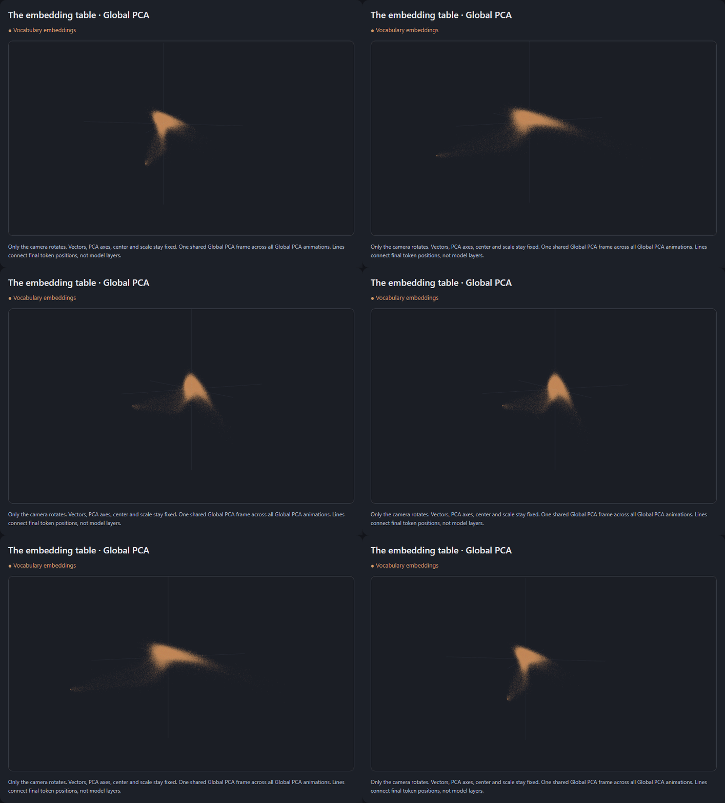
The embedding table already encodes learned relationships between tokens. Training shapes these vectors through patterns in how tokens are used, giving the model a meaningful starting point for understanding and processing text. The layers then refine those starting representations using the context available at each position. A whole conversation contains many token states, rather than one single 2,048-number description.

The shape of English

I started with 900 English question-and-answer examples across 100 topics, all processed by the same frozen model.

Each token begins with a learned vector from the embedding table. Qwen’s layers update its representation using the context available at that position. I recorded the final token states and normalized their lengths so the visualization compared directions.

In the pictures below, the orange cloud still shows the input embeddings as individual points. The colored lines connect the final token states from each conversation example. Each line segment joins the state at one token position to the state at the next, tracing a path through this projected space as the question and answer progress. Many conversation paths are shown together at the same time. These lines connect discrete saved states in text order; they do not show a token’s journey through the model’s layers.

To keep the comparison fair, I computed one Global PCA frame using the vocabulary embeddings and all the conversation averages. I then revealed the datasets one at a time. Adding a language to these pictures changes visibility, while the global axes stay fixed.

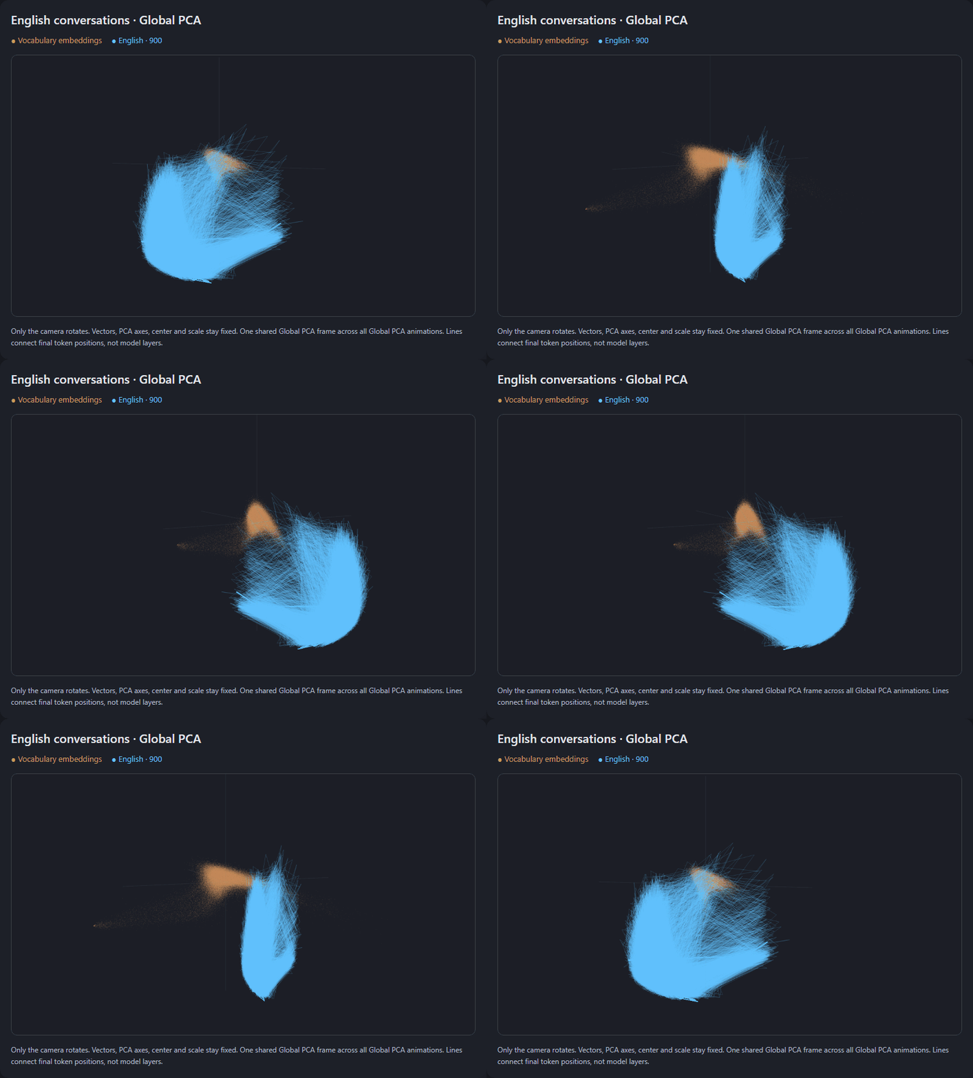
Across a hundred topics, the English states seemed to occupy a thin sheet. As the camera turned, a broad shape narrowed almost to an edge.

That impression survived measurement: a best-fitting plane contained approximately 99.3% of the English token states’ variation within this 3D projection.

It was tempting to interpret the sheet as evidence that the model had compressed an enormous variety of conversations into a remarkably simple surface. Before accepting that explanation, I wanted to change something more fundamental than the topic.

Does language change the shape?

I introduced Chinese versions of the same topics and question intents, then let Qwen generate its answers independently.

The pink states appeared in a neighboring region, visibly offset from English.

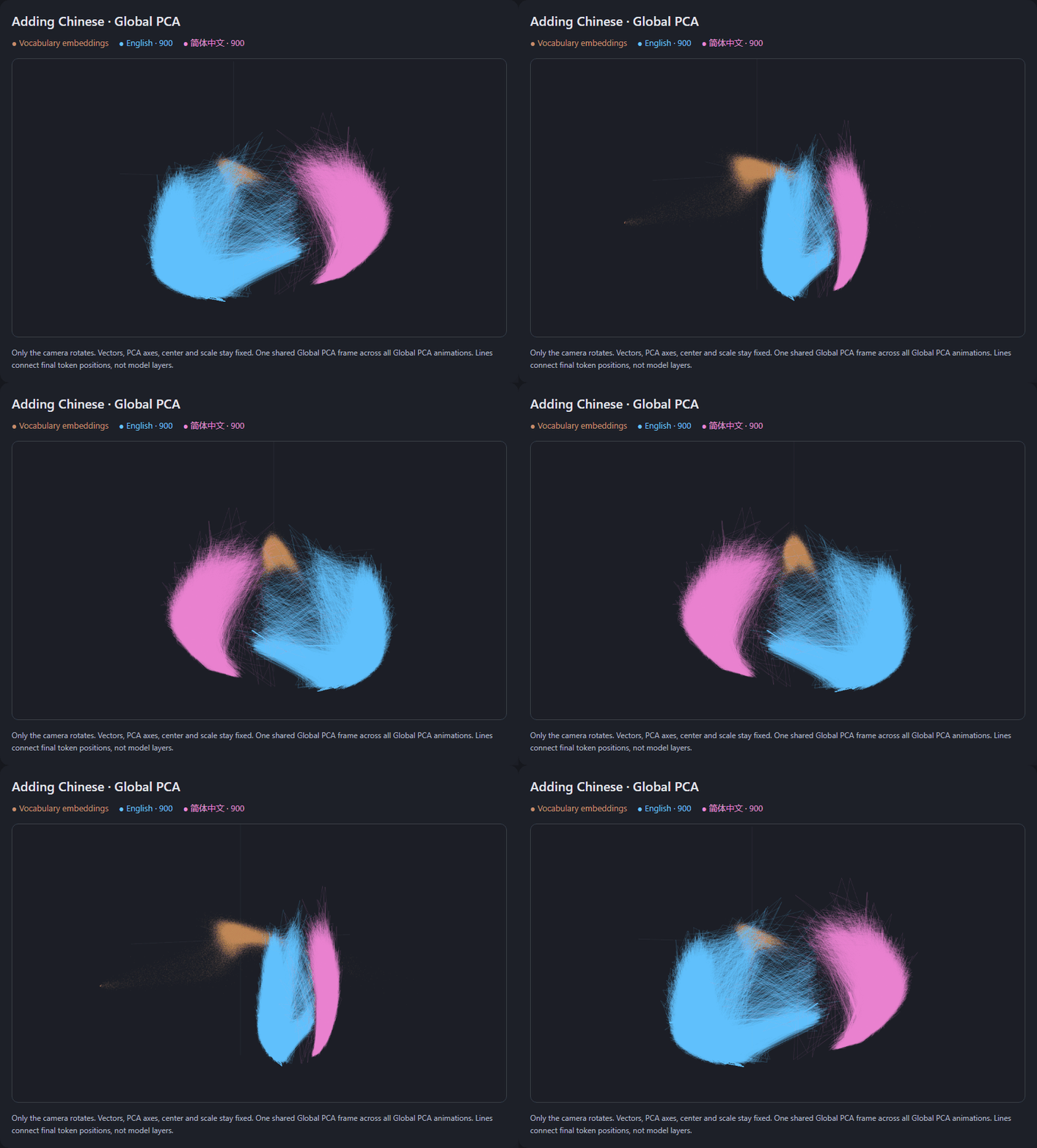
The separation made an abstract question tangible. A representation can carry information about both the subject being discussed and the language used to discuss it.

If similar questions in Chinese and English occupy different regions, what does that separation represent? The idea itself? The writing system? The vocabulary and structure the model needs to produce its answer?

The geometry alone could not disentangle those possibilities. Language, script, tokenization, wording, and answer quality all changed together in this experiment.

Perhaps expecting a representation to contain “pure meaning,” cleanly detached from the form used to express it, was already an assumption I had brought to the map.

Then I added German and Croatian.

These offered a useful comparison: two more natural languages using Latin-script writing.

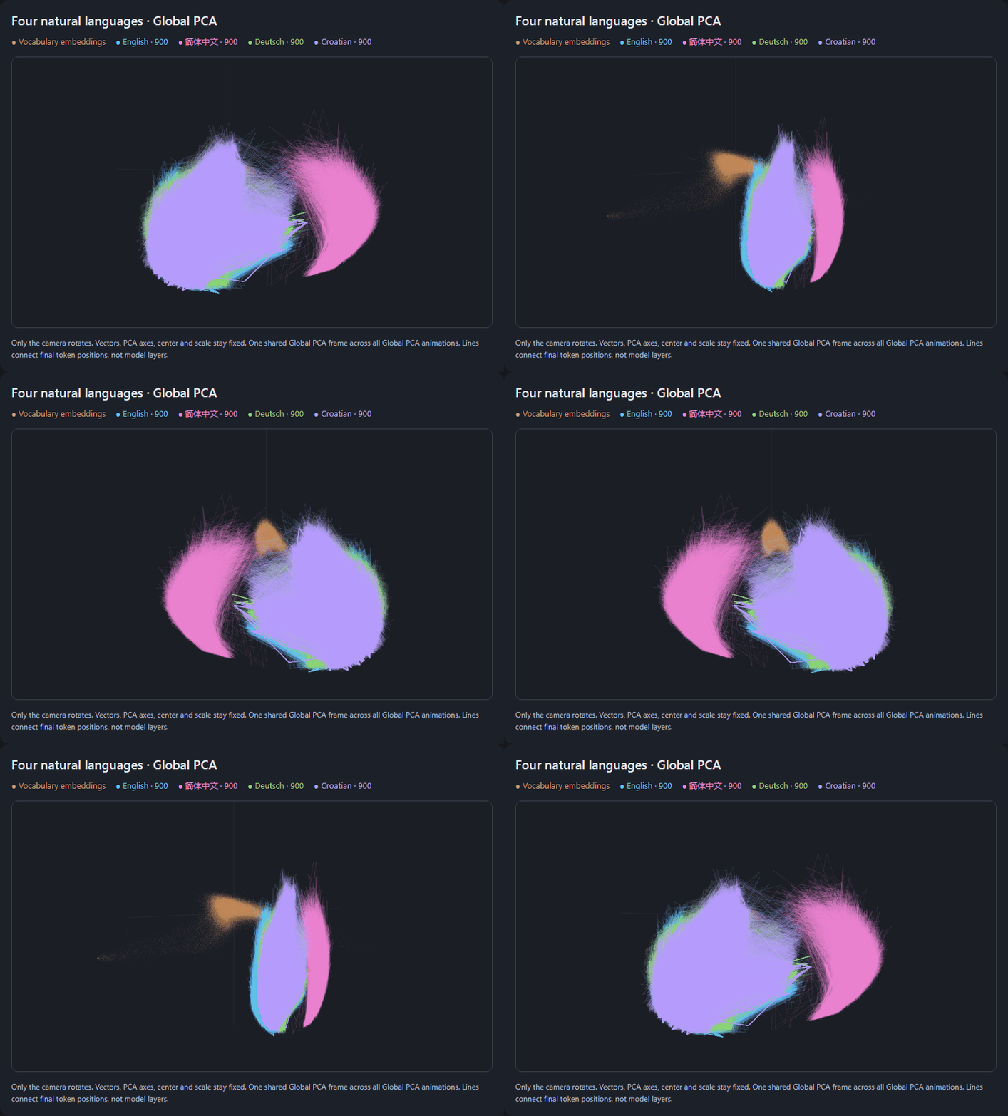
German and Croatian occupied the broad neighborhood of English, with substantial overlap. Chinese remained more visibly offset in this view.

The picture suggested overlapping regions with different centers and shapes. It did not establish separate language compartments throughout the model’s entire residual space.

The shapes also reflected the practical construction of the examples. Croatian responses contained many more Qwen tokens than the English responses. More token states produce more points and line segments. A larger or denser patch therefore cannot be read directly as greater knowledge or capacity.

I was beginning to distinguish the appearance of a region from the explanations I wanted to attach to it.

Where code fits

Next came 90 Python coding examples: list processing, sorting, binary search, graph traversal, JSON, dates, matrices, recursion, and classes.

Would code form a distant island?

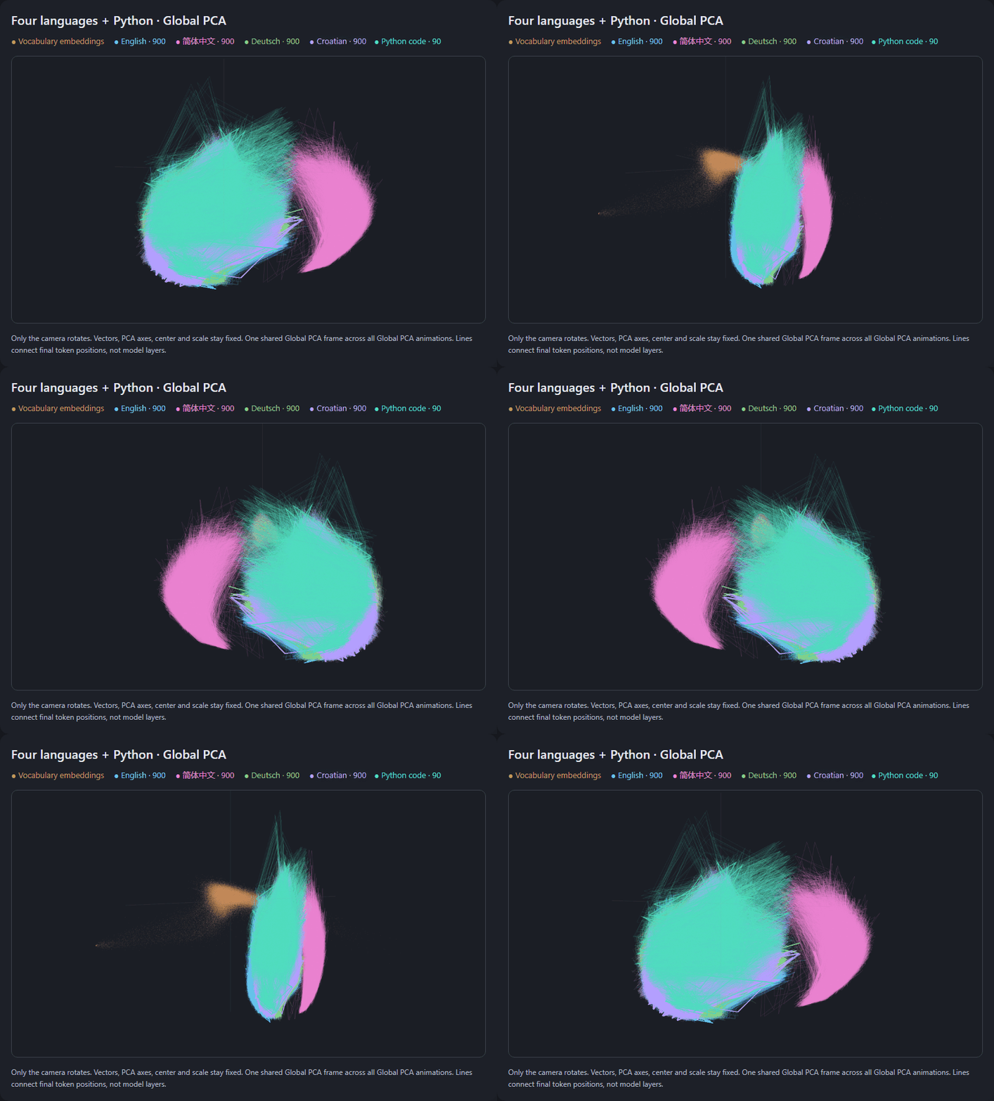
Code appeared in the same broad neighborhood as English and the other Latin-script datasets. Hiding the other languages makes that visual comparison easier to inspect.

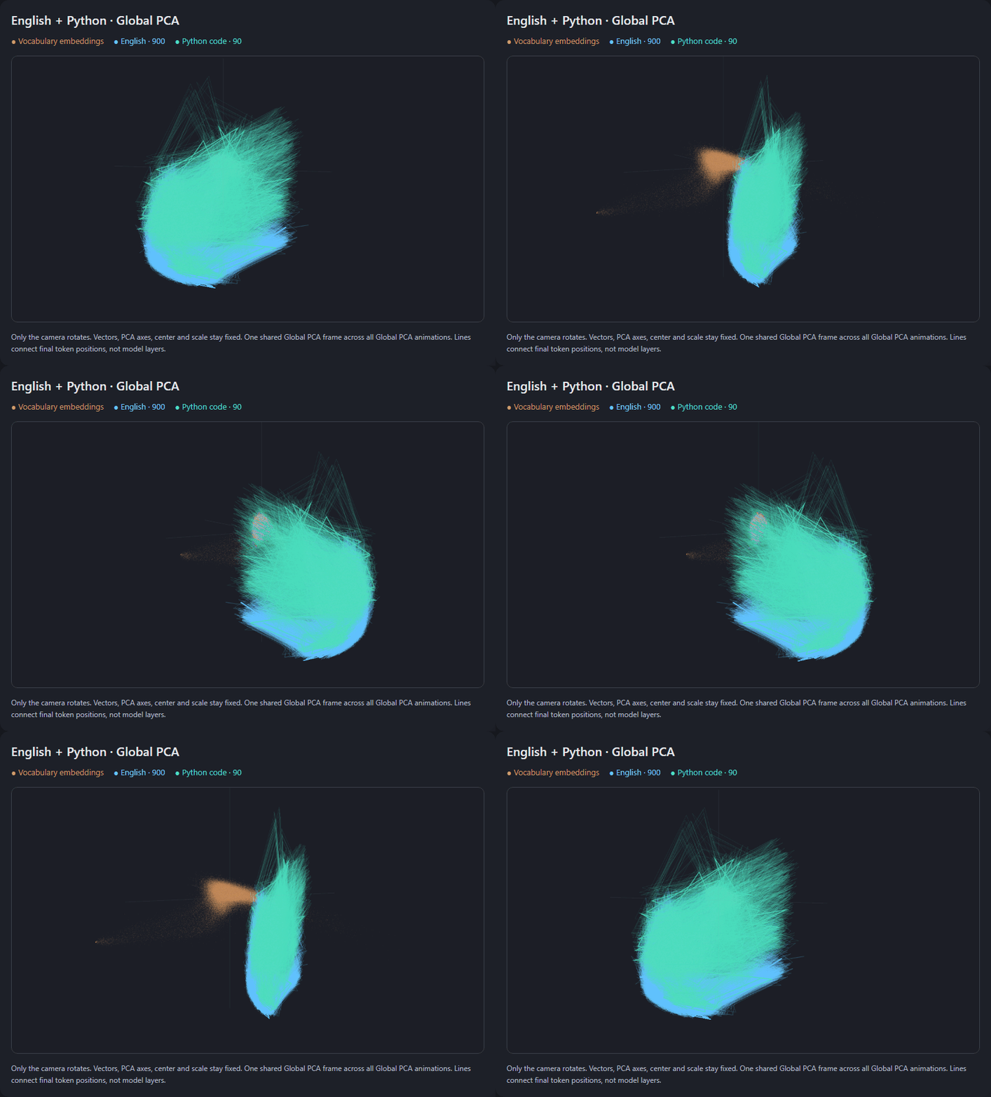
That proximity was interesting, but the construction of the dataset mattered. Python uses English-like keywords alongside punctuation and operators, and each plotted example included its English question as well as its code answer.

Even “close” needed a definition. A simple distance comparison between the projected conversation averages placed the coding dataset closer to Croatian and German than to English. Being in English’s broad visual neighborhood and having English as its closest numerical neighbor were different claims.

When we call code a language, are we talking about its symbols, its structure, or its purpose? In this experiment, several of those properties were entangled in the same examples.

Changing the window

The Global PCA fit contained 151,936 normalized input embeddings and 3,690 conversation averages. Vocabulary embeddings accounted for roughly 98% of its fitting points.

PCA does not know which observations I consider most interesting. It finds directions that explain variation in the data I give it.

So I tried Conversation PCA: choose the directions using the conversation averages alone, then project the same saved token states and embedding table into that new frame.

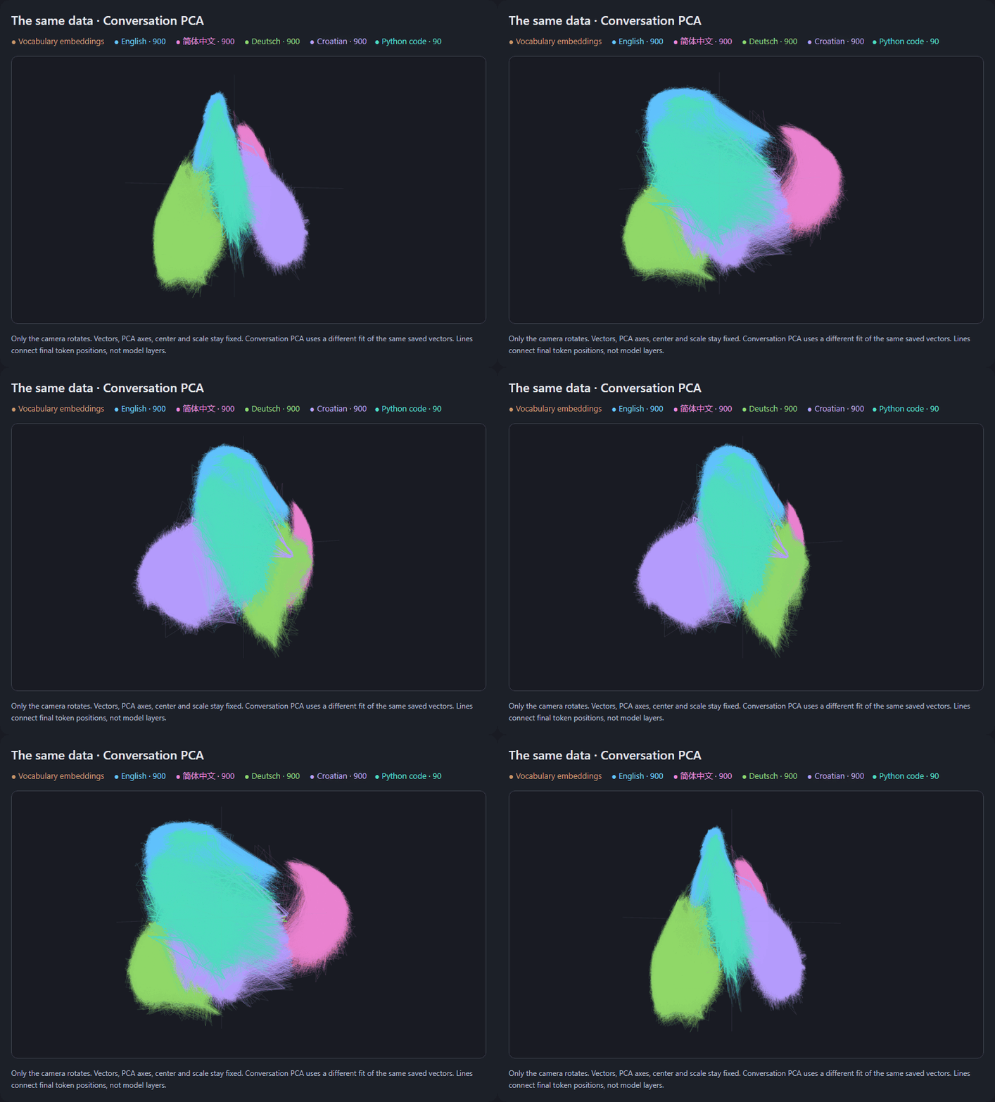
The relationships became visible through a different geometry. German and Croatian spread into more distinguishable regions, while substantial overlap remained.

The change was measurable. The three Conversation PCA directions captured 80.1% of the variation between conversation averages. The three Global PCA directions captured 42.4% of that same average-vector variation.

Those percentages describe conversation averages. The token paths are shown in the resulting frame, but they were not the points used to fit it.

This exposed an important choice inside the visualization: what should the map be optimized to preserve? A vocabulary-oriented frame and a conversation-oriented frame can emphasize different relationships in the same underlying representations.

What the map leaves out

I checked the apparent flatness against all 264,571 final token states in their original 2,048-dimensional space.

Measurement	Result
Visible 3D variation contained in a best-fitting plane	99.7%
Full token-state variation captured by the displayed Global PCA axes	17.6%
Full variation captured by the best possible 2D plane fitted in 2,048 dimensions	28.7%
PCA directions needed to retain 90% of full token-state variation	684

The visible sheet contained almost all the variation in the 3D view, but that view left out 82.4% of the original variation. Even the best plane fitted in the full space captured only 28.7%, with a similar 28.4% on held-out topics.

At the same time, 17.6% in three directions is a substantial concentration. If variation were spread equally across all 2,048 directions, three would account for only about 0.15%. The observed share was roughly 120 times that reference.

The axes strongly tracked language, with topic structure still present after accounting for language. This connects to earlier research on language-sensitive and shared geometry in multilingual models. These measurements describe associations in this dataset and projection.

In this post, we took an exploratory look at how conversations appear in the residual vector space an LLM uses to process text. In our three-dimensional view, thousands of conversations formed thin, overlapping sheets. Different languages and code traced paths through partly shared regions, revealing a common geometric structure across the examples.